Batching

In scenarios where numerous small simulations are required, for instance, for statistical analysis or parameter exploration, running these simulations sequentially might not be the most efficient approach. Let us assume a single simulation takes a time T to complete. If we need to perform N simulations sequentially, the total time required would be TN. However, since GPUs are not fully utilized during each small simulation, this presents an opportunity to execute multiple simulations simultaneously on the same GPU.

We want to group simulations into batches, where each batch, of size N_S, contains enough simulations to fully utilize the capacity of the GPU. Ideally, the execution time for a batch of N_S simulations should be approximately equal to the time for a single simulation (T). Therefore, the total number of batches needed would be approximately N_B ≈ N/N_S, and the overall execution time becomes ≈ TN_B ≃ TN/N_S < TN. In certain systems, batch sizes could be as large as N_S ≈ 100, leading to significant efficiency gains.

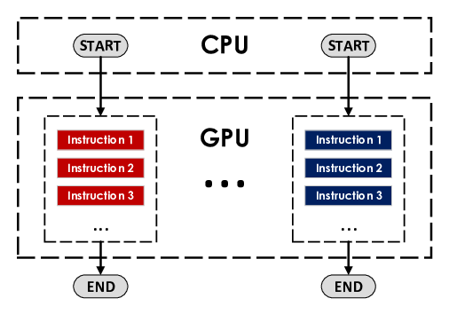
However, the actual implementation of this batching on GPUs can be challenging due to their inherent hardware design. When different simulations are executed on the same GPU, their instructions tend to become serialized rather than parallelized. This effect is illustrated in Fig. 1. In Panel A, two simulations are executed sequentially, with each running its instructions in order. In contrast, Panel B shows what happens when two simulations are run simultaneously on the GPU: instructions from each simulation are executed in an alternating pattern [This explanation is a simplification; the process involves more complexities and details]. Unfortunately, this interleaving of instructions disrupts the potential benefits of simultaneous execution, as it does not lead to a significant reduction in total computational time.

Illustration of default multitasking on GPU. A) Two different programs are executed sequentially. First, the instruction set of the first program is evaluated and once it is finished, the instructions of the second program are evaluated. B) Both programs are executed at the same time. The instructions that compose both programs are evaluated alternately, the time needed to execute the two programs in this way is similar to that required in A.

To overcome the challenges of multitasking inefficiencies on GPUs, NVIDIA introduced the Multi-Process Service (MPS). MPS facilitates the concurrent execution of multiple programs on the GPU, but it comes with certain limitations. Each simulation running on the GPU requires execution by a CPU core, thus making CPU cores a bottleneck in scenarios with numerous simulations. There is also a cap on the number of processes that can run simultaneously on the GPU. Memory usage scales linearly with the number of simulations; each new simulation added demands a similar amount of memory. Another constraint is that different instances within MPS do not easily exchange information between them. This restriction leads to problems for algorithms that require inter-batch communication. One of the major complications with MPS is its requirement for prior configuration through software, as it is not available by default. In high-performance computing environments like computing clusters, configuring MPS can be quite complex. Consequently, it is not widely used in such environments due to the complexity of its configuration.

CUDA MPS illustration. When using CUDA MPS, each program is associated with a different process and can run concurrently sharing GPU resources.

UAMMD-structured addresses the challenges of GPU multitasking by introducing an efficient batching system. This system enables simultaneous execution of any number of simulations, maximizing the capacity of the GPU without being limited by the number of CPU cores, as it functions as a single process. One of the key advantages of the batching system of UAMMD-structured is its minimal memory usage. This efficiency is achieved by sharing large data structures, like neighbor lists, across multiple simulations. Such an approach is particularly beneficial for simulations involving memory-intensive potentials, including tabulated potentials and increasingly popular neural network-based potentials. The latter, already implemented in programs like LAMMPS, could potentially be extended to UAMMD-structured. The system design also enables easy exchange of information between different batches, which can be used to implement algorithms that require multiple independent simulations, such as parallel tempering. To utilize the batching system in UAMMD-structured, we need to chose which particles belong to different batches. This categorization is done in the structure Section:

state:
  labels: ["id", "position"]
  data:
    - [0, [1.6, 2.7, 3.3]]
    - [1, [2.5, -3.7, -1.9]]
    - [2, [-3.3, 1.0, 2.1]]
    - [3, [1.5, -1.1, 0.2]]
    - [4, [2.3, 1.5, 2.8]]
    - [5, [-1.5, 1.7, -2.1]]
    - [6, [-2.8, 1.3, 1.7]]
    - [7, [4.5, 1.3, 1.2]]
    # ...

topology:
  structure:
    labels: ["id", "type", "batchId"]
    data:
      - [0, "A", 0]
      - [1, "A", 0]
      - [2, "A", 0]
      - [3, "A", 0]
      - [4, "A", 1]
      - [5, "A", 1]
      - [6, "A", 1]
      - [7, "A", 1]
      # ...

In this example, alongside the type in the structure, an additional column named “batchId” is included. This “batchId” indicates the batch of each particle, integrating it into the hierarchical structure: particle ⊂ residue ⊂ chain ⊂ model ⊂ batch. When two particles have different IDs in this column (i.e., different “batchId”), UAMMD-structured handles them as belonging to separate batches. This ensures that these particles do not interact with each other during simulations. For some types of potentials, interaction parameters can be tailored based on the “batchId”:

topology:
  forceField:
    # ...
    nl:
      type: ["VerletConditionalListSet", "all"]
      parameters:
        cutOffVerletFactor: 1.2
    batched_LennardJones:
      type: ["NonBonded", "LennardJonesType2"]
      labels: ["name_i", "name_j", "epsilon", "sigma", "batchId"]
      data:
        - ["A", "A", 1.0, 1.5, 0]
        - ["A", "A", 3.0, 3.5, 1]
      parameters:
        condition: "all"
        cutOffFactor: 2.5
    # ...

Such a structure enables encapsulating a broad range of situations within a single batch. For interactions where parameters are associated with particle IDs, like bonds, setting different parameters for batches effectively means assigning different parameters for each listed interaction.

The implementation of batches in UAMMD-structured is software-based. Specifically, each component of UAMMD-structured, including interactions, simulation steps, and others, must handle different batches. This requirement is the primary limitation of the batching system of UAMMD-structured compared to hardware-based batching methods like MPS.

To effectively utilize batching, UAMMD-structured not only implements it at the code level but also integrates it into the pyUAMMD Python library. As we will discuss in the following section, pyUAMMD includes a mechanism to automatically combine different simulations into a single simulation.

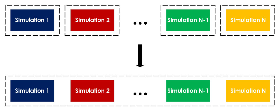
UAMMD-structured batching is done by combining the different inputs from different simulations into a single input, i.e. into a single simulation. To ensure that particles belonging to different simulations do not interact with each other, a different batchId is associated with them.

The batching implementation in UAMMD-structured is composed of two integral parts: the primary functionality within UAMMD-structured itself, which ensures that particles from different batches do not interact during simulation, and the pyUAMMD library, which provides an easy combined input generation.

As mentioned previously, batching in UAMMD-structured operates through software, requiring each component to recognize and handle particles with distinct “batchId” values. However, this software-based approach limits the applicability of batching with certain interaction types and integrators. Particularly, batching is incompatible with components that involve hydrodynamic interactions and electrostatic interactions. This is because, for these particular features, UAMMD-structured mainly serves as a wrapper for UAMMD, which does not inherently support batching. Therefore, using batching with these incompatible components results in an error and consequent termination of the simulation.

Regarding interactions of UAMMD-structured, handling batching is relatively straightforward for bonds, many-body bonds and AFM, as long as two particles from different batches are not part of the same bond or belong to the same AFM. This condition is verified prior to the simulation start, and an error is issued if the condition is violated. For external interactions is similar, no additional considerations are needed, since this kind of interaction involves one particle only. For short-range interactions, batching is implemented effectively due to conditioned Verlet lists. This is done adding a simple check: if particles i and j belong to different batches then they can not become neighbors.

The approach to simulation steps in the presence of batches is slightly different. Since these steps are not crucial to the core simulation (being executed periodically), they are implemented by modifying the input. This task is handled by the pyUAMMD library, which organizes simulation steps by creating groups for each batch and applying the steps to different batches. While this method does not run simulation steps in parallel, it allows them to function effectively in simulations with multiple batches.

Through these procedures, a large number of simulations can be run simultaneously in UAMMD-structured. When smaller simulations are combined into batches, the total execution time remains essentially unchanged. This holds true until the combined simulation reaches a size that fully utilizes the resources of the GPU. Even at this point, a modest improvement in performance is achieved because certain operations, like kernel preparation, occur concurrently for all simulations.

In scenarios where there are numerous small simulations to be executed, the most effective strategy involves distributing these simulations across available GPUs. This is done by dividing the total number of simulations by the number of GPUs, forming batches accordingly. Each batch is then assigned to a different GPU for parallel processing. This batching approach is especially beneficial when dealing with a large number of simulations, each of which is relatively small in size.

It is also worth noting that this approach fills a gap often overlooked by current simulation environments like GROMACS, LAMMPS, and OPENMM. These platforms tend to focus on simulating increasingly larger systems, sometimes neglecting the frequent need for multiple smaller simulations. Furthermore, as GPU technology continues to advance, so the definition of what constitutes a ‘small’ simulation is constantly expanding.