Short Range
Short-range interactions are employed for modeling a wide range of physical phenomena. The Lennard-Jones potential, for example, is extensively used to simulate interactions between uncharged particles. Moreover, the Debye-Hückel potential plays a critical role in modeling charged particles within saline solutions. These potentials, while grounded in physical concepts, are also employed as conceptual models. They are often used to hypothesize about the nature of the studied phenomena, particularly when the exact physical underpinnings are not well-defined. This approach is exemplified by the Lennard-Jones potential, which is employed to represent particles with steric interactions and short-range attractive forces. Additionally, it serves as a foundational model, frequently modified to introduce other effects, showcasing its versatility as a fundamental tool in physical system modeling.
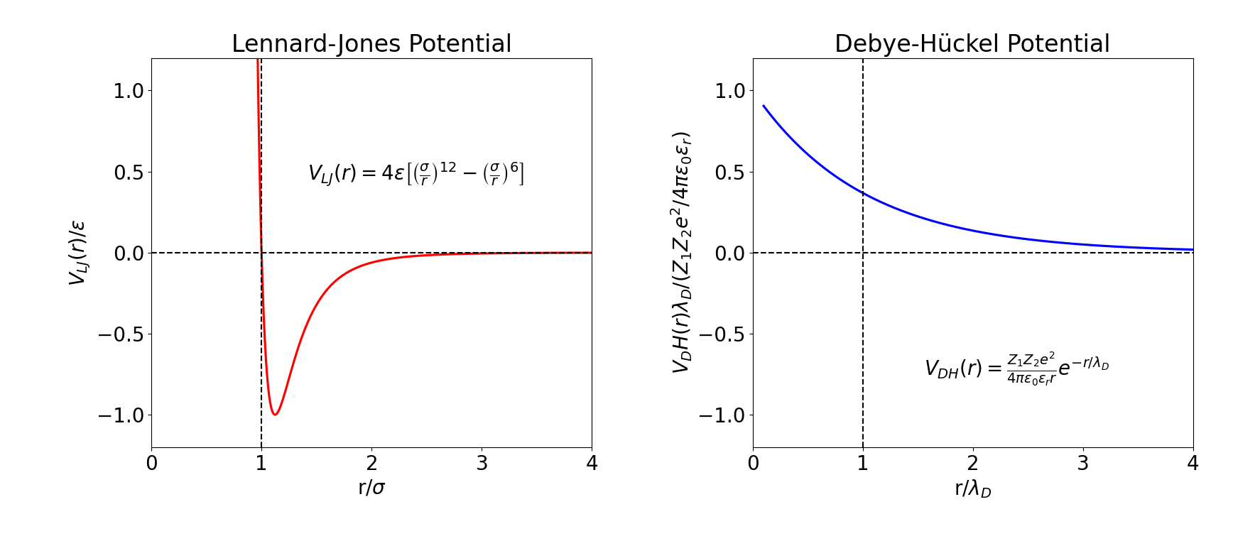
Lennard-Jones Potential (Left) and Debye-Hückel Potential (Right). These potentials are characterized by rapid decay, qualifying them as short-range potentials.
While multi-body short-range potentials are more general (naturally resulting from exact coarse graining theory) and used in some applications, this discussion focuses on two-body (pairwise) potentials. The application of a truncation to these potentials leads to the definition of a cutoff radius r_cut, where U(r) = 0 for all r > r_cut. The choice of r_cut is potential-specific and often depends on the parameters within the model. For instance, with the Lennard-Jones potential, a typical cutoff radius is r_cut = 2.5σ, balancing computational efficiency with physical accuracy.
From a computational standpoint, short-range potentials offer several advantages. In contrast to long-range potentials, where the interaction of a particle with all others must be calculated, short-range interactions simplify computations significantly. Generally, there are three main approaches to computing long-range interactions: N-body approximations, Ewald summation, and the fast multipole method, among others. The first two are implemented in UAMMD and in particular Ewald summation is used for computing electrostatic interactions that will be introduced later. However, a common trait among these methods is their relatively high computational cost, exceeding O(N). In contrast, for short-range interactions, it is possible to construct structures, commonly referred to as neighbor lists, which significantly reduce computational complexity to an O(N) level. These neighbor lists efficiently manage the interactions between particles by only considering those within a predetermined distance. This approach ensures that only the most relevant interactions are computed, thereby saving valuable computational resources and time. This efficiency is particularly advantageous in simulations involving a large number of particles, where every reduction in computational load can lead to significantly faster and more efficient simulations.
In our context, we introduce neighbor lists, neighbor lists are understood as structures that enable access to all neighbors of a given particle. Specifically, for a particle i, these lists include particles j for which the condition distance(i, j) < r_neighbors holds, with r_neighbors ≥ r_cut. This criterion ensures that all the particles within the interaction range defined by the cutoff radius r_cut are included in this list.
Various algorithms exist for constructing neighbor lists in computational simulations. The straightforward approach would involve calculating the distances between all particle pairs and then, for each particle i, assembling a list of neighbors comprising those particles j that lie within a distance less than r_cut. However, this method is computationally expensive, characterized by a O(N^2) complexity, akin to the traditional N-body approach.
To optimize this process, more efficient algorithms have been developed, one of which is the cell list method. This method hinges on subdividing the simulation space into a grid of cells. The number of cells in each dimension α (where α includes x, y, and z dimensions) is determined by dividing the simulation volume length L_α by the cutoff radius r_cut and taking the floor value: n_α = floor(L_α / r_cut). Consequently, the total number of cells is given by N_cells = n_x · n_y · n_z.
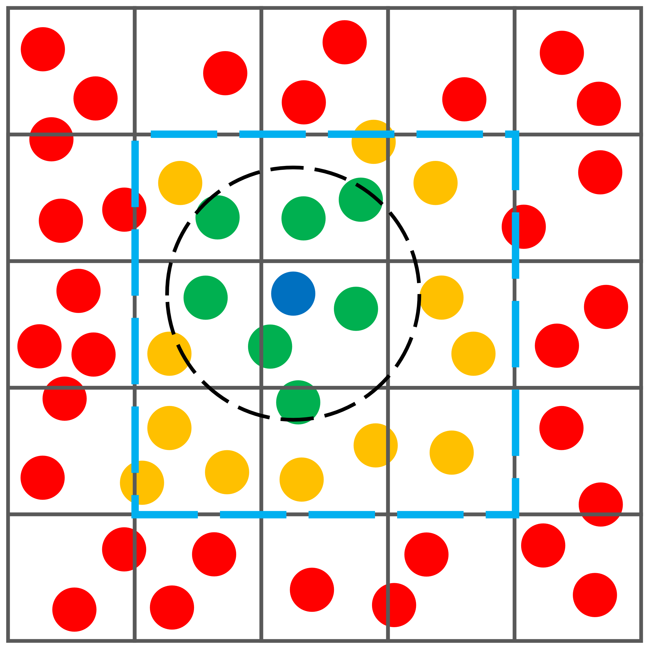
Example of a two-dimensional cell list. In this example, the size of each cell is w≈r_cut. When determining the neighboring particles of a certain target particle (the blue particle in the figure), we only check those particles that are located in the same cell as the evaluated particle and in the neighboring cells (within the dashed blue square in the figure). Particles that are not found in these cells (the red particles in the figure) are not considered as candidates, which greatly reduces the compilation time. Of the particles we check, only those that are located at a distance less than r_cut (the green particles in the figure) are considered neighbors, so the remainder particles in the neighbor cells (orange particles in the figure) are not considered when the potential is computed.
In this cell list approach, each particle is assigned to the cell it occupies in space. The neighbor list for a particle i is then constructed by examining particles j not only in the same cell as i but also in adjacent cells, respecting periodic boundary conditions. A particle j is added to the neighbor list of i if the distance distance(i, j) is less than r_cut. This approach drastically reduces the number of distance computations. Assuming a uniform distribution of particles, the average number of particles per cell is N_ppc = N / N_cells. In a 3D space, each cell interacts with its own and the 26 adjacent cells, leading to an average of N_checks = 27 · N_ppc = 27 · N / N_cells distance checks per particle, a significant reduction from the N^2 checks required by the direct pairwise comparison method.
Although the cell list method considerably lowers computational complexity, it does have limitations, particularly in GPU-based implementations. While in CPU implementations, the linked cell approach allows for dynamic updating of cells as particles move, the GPU requires a complete reconstruction of the list at each integration step due to the simultaneous movement of all particles. This need for continual reconstruction introduces additional computational overhead.
To efficiently manage the need for frequent reconstruction of neighbor lists in simulations, the Verlet list approach is utilized. The key principle of Verlet lists is to minimize the continuous rebuilding of these lists. This objective is achieved by creating a neighbor list with an enlarged radius, termed the Verlet radius, r_Verlet, which is larger than the cutoff radius, r_cut. As a result, the neighbor list constructed using r_Verlet remains valid for the interactions within the range of r_cut. In essence, for every particle i, all other particles j that satisfy the condition distance(i, j) < r_cut are included in the neighbor list of i. This inclusion holds as long as no particle travels beyond a distance greater than r_max from its initial position when the list was generated. The distance r_max is defined as follows:
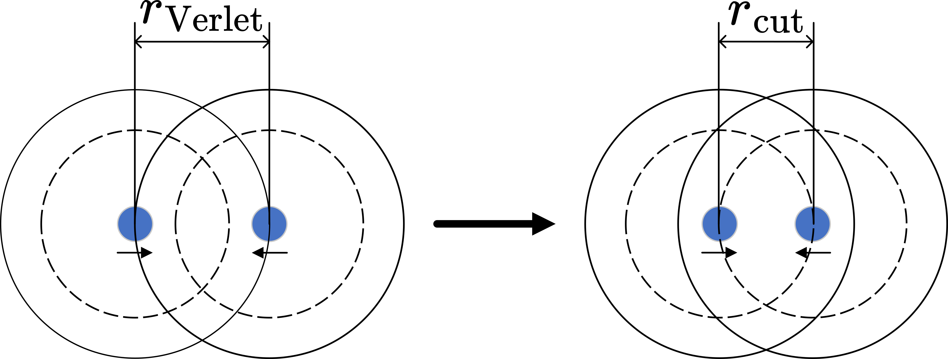
Initially, two particles lie outside the neigbhor list of each other, separated by the Verlet distance r_Verlet, which is greater than the cutoff radius r_cut. Over time, if they move closer such that their separation is less than r_cut, they should be included in neighbor list of each other for interaction calculations. The maximum allowable movement without updating the Verlet list is r_max = (r_Verlet - r_cut)/2, ensuring all potential interactions are accounted for within the simulation timeframe.
This particular distance is calculated based on the worst-case scenario, as illustrated in Fig. Here, two particles initially distanced at r_Verlet and therefore not in neighbor lists of each other, start moving towards one another in opposite directions. After some time, their distance diminishes to r_cut, at which point their interaction becomes relevant, necessitating their inclusion in the neighbor lists of each other. The total distance traversed by the particles in this scenario is r_Verlet - r_cut, and consequently, each particle travels a distance given by the equation above. Since we cannot conclusively determine whether this situation will occur, the Verlet list must be reconstructed whenever a particle moves the distance defined by the equation.
In summary, we generate the cell list for a radius larger than the cutoff radius, denoted as r_Verlet (note that we use cell lists, but other algorithms could be used for constructing the neighbor list; the Verlet list is an algorithm to trigger the list reconstruction, not for the construction itself). Each time we update the positions of the particles, we check if they have moved a distance greater than r_max compared to the position when the list was built. If so, we reconstruct the list.
The key parameter in Verlet lists is the Verlet radius, r_Verlet. As we increase the radius, we also increase the number of particles we need to check when evaluating an interaction. Conversely, we can perform more updates before needing to reconstruct the list. Therefore, the efficiency of this approach depends quite a bit on the specific system; its density, diffusion, etc.
Let us now consider how Verlet lists behave for certain types of potentials, specifically examining their behavior for certain coarse-grained models. We will use a protein model as an example, but the principles can be generalized to many other cases. In these models, it is common to employ different types of interactions for particles within the same structure “intra” interactions and those involving interactions between particles from different structures, “inter” interactions, [By a common misuse of language, the terms “intramolecular” and “intermolecular” are often employed, even when not dealing with molecules per se]. This situation is depicted in Fig.
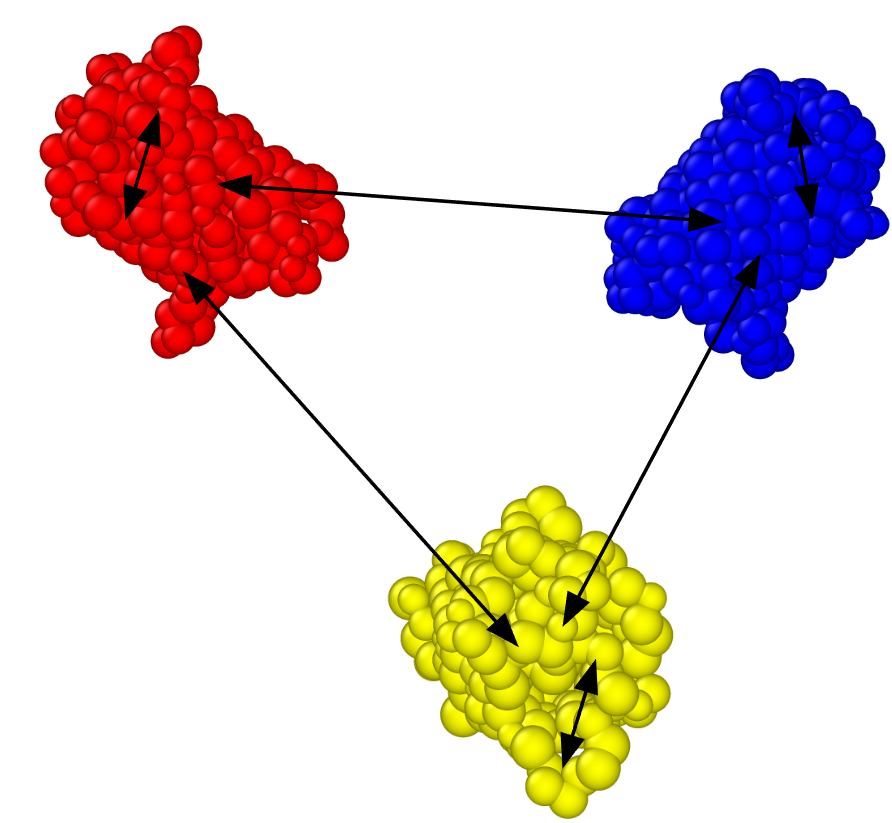
Coarse-grained models with three copies of a protein (GFP), each colored differently. Interactions involving particles of the same color (same structure) engage with a different potential than those involving particles of different colors (different structures).
The approach combining cell lists and Verlet lists encounters challenges in handling these types of interactions. The feasible solution involves evaluating each interaction to determine the appropriate potential. This process, particularly on GPUs, faces difficulties due to the SIMD architecture. It causes significant divergence in the code, adversely affecting performance. Furthermore, this approach limits the reusability of interactions because it necessitates the implementation of distinct potentials for each specific scenario. For instance, consider a scenario where the inter interactions are modeled using a Lennard-Jones potential, and the intra interactions employ a WCA-type potential. In such a case, it becomes essential to define a unified potential capable of appropriately applying either the Lennard-Jones or WCA interaction, based on the particle pairs (intra/inter). Ideally, implementing a versatile potential system that allows for selective application to various particle pairs would be more efficient, reducing the need for extensive coding.
The available short-range potentials are listed below: